
John Avina, Director
Abraxas Energy Consulting
October 20, 2011
Abstract
Utility Bill Tracking systems are at the center of an effective energy management program. However, some organizations spend time and money putting together a utility bill tracking system and never reap any value. This paper presents three utility bill analysis techniques which energy managers can use to arrive at sound energy management decisions and achieve cost savings.
Introduction
Utility bill tracking and analysis is at the center of rigorous energy management practice. Reliable energy management decisions can be made based upon analysis from an effective utility bill tracking system. From your utility bills you can determine:
- Whether you are saving energy or increasing your consumption
- Which buildings are using too much energy
- Whether your energy management efforts are succeeding
- Whether there are utility billing or metering errors
- When usage or metering anomalies occur (ie. when usage patterns change)
Any energy management program is incomplete if it does not track utility bills. Equally, any energy management program is rendered less effective when its utility tracking system is difficult to use or does not yield valuable information. In either case, fruitful energy savings opportunities are lost.
Many practical energy managers make the smart choice and invest in utility bill tracking software, but then fail to recover their initial investment in energy savings opportunities. How could this be?
This paper introduces three simple and useful procedures that can be performed with utility bill tracking software. Just performing and acting upon the first two types of analysis will likely save you enough money to pay for your utility bill tracking system in the first year. The three topics are Benchmarking, Load Factor Analysis, and Weather Normalization as shown in Table 1.
TABLE 1. 3 UTILITY BILL ANALYSIS TECHNIQUES
| Benchmarking |
|
| Load Factor Analysis |
|
| Weather Normalization |
|
Benchmarking
Let’s suppose you were the new energy manager in charge of a portfolio of school buildings for a district. Due to a lack of resources, you cannot devote your attention to all the schools at the same time. You must select a handful of schools to overhaul. To identify those schools most in need of your attention, one of the first things you might do is find out which schools were using too much energy. A simple comparison of Total Annual Utility Costs spent would identify those buildings that spend the most on energy, but not why.
Figure 1: Comparison of Total Annual Utility Costs
As seen in Figure 1, Santa Rosa Elementary School (ES), San Simeon ES and San Gabriel ES cost the most to operate, while San Luis Obispo ES and Creston ES cost the least. But these three schools may not be the best schools to work on first. Most likely the buildings that spend the most on energy are the largest buildings in the portfolio. It would be wiser to find those buildings that spend the most per square foot per year. This process is referred to as benchmarking, and is presented in Figure 2.
Figure 2: Comparison of Total Annual $ per Square Foot
Figure 2 shows the same schools, but the costs are divided by square footage (SQFT). Santa Rosa and San Simeon ES are still the best targets, but San Gabriel ES is actually one of the more efficient schools. Instead San Luis Obispo ES is the third most wasteful school on a $/SQFT basis. From this, we can also see that the most inefficient schools cost about 30% more to operate than the most efficient schools.
Benchmarking Different Categories of Buildings
When benchmarking, it is also useful to only compare similar facilities. For example, if you looked at a school district and compared all buildings by $/SQFT, you might find that the technology centers administration buildings were at the top of the list, since administration buildings and technology centers often have more computers and are more energy intensive than elementary schools and preschools. These results are expected and not necessarily useful. For this reason, it might be wise to break your buildings into categories, and then benchmark just one category at a time.
Different Datasets
You can benchmark your buildings against each other (as we did in our example) or against publicly available databases of similar buildings in your area. Energy Star’s Portfolio Manager allows you to compare your buildings against others in your region. Perhaps those buildings in your portfolios that looked the most wasteful are still in the top 50th percentile of all similar buildings in your area. This would be useful to know.
Setting Realistic Targets Using Benchmarking
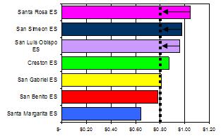
Figure 3: Realistic goal for energy mangers to meet.
Occasionally, management decides that their organization needs to save some arbitrary percentage (5%, 10%, etc.) on utility costs each year. Depending upon the goal, this can be quite challenging, if not impossible. Energy managers can use benchmarking to guide management in setting realistic energy management goals, as shown in Figure 3. For example, our school district energy manager might decide to create a goal that the three most energy consuming schools use only $0.80/SQFT. Since this is about as much as the lowest energy consuming schools are currently using, this could be an attainable goal.
If you can find a dataset, you may also be able to benchmark your buildings against a set of similar buildings in your area and see the range of possibilities for your buildings. In any case, benchmarking will focus your energy management efforts and provide realistic goals for the future.
Rules of Thumb
New energy managers often search for a “rule of thumb” to use for benchmarking. An example could be: “If your building uses more than $2/SQFT/Year then you have a problem.” Unfortunately, this won’t work. Different types of buildings have different energy intensities. Moreover, different building locations will require differing amounts of energy for heating and cooling. In San Francisco, where temperatures are consistently in the 60s, there is almost no cooling requirement for many building types; whereas in Miami, buildings will almost always require cooling. Different building types, with their characteristic energy intensities, different weather sites, and different utility rates all combine to make it hard to have rules of thumb for benchmarking. However, energy managers whose portfolios are all close by, can develop their own rules of thumb. These rules will most likely not be transferable to other energy managers in different locations, with different building types, or using different utility configurations.
Benchmarking Buildings in Different Locations
There are some complications associated with benchmarking. Suppose you were the energy manager of a chain store, and you had buildings in different national locations. Then benchmarking might not be useful in the same sense. Would it be fair to compare a San Diego store to a Chicago store, when it is always the right temperature outside in San Diego, and always too hot or too cold in Chicago? The Chicago store will constantly be heating or cooling, while the San Diego store might not have many heating or cooling needs. Comparing at $/SQFT might help decide which store locations are most expensive to operate due to high utility rates and different heating and cooling needs.
Some energy analysts benchmark using kBtu/SQFT to remove the effect of utility rates (replacing $ with kBtu). Some will take it a step further using kBtu/SQFT/HDD[1] to remove the effect of weather (adding HDD), but adding HDD (or CDD) is not a fair measurement, as it assumes that all usage is associated with heating. This measurement also does not take into account cooling (or heating) needs. Many thoughtful energy managers shy away from benchmarking that involves CDD or HDD.
Different Benchmarking Units
Another popular benchmarking method is to use kBtu/SQFT (per year), rather than $/SQFT (per year). By using energy units rather than costs, “rules of thumb” can be created that are not invalidated with each rate increase. In addition, the varying costs of different utility rates does not interfere with the comparison.
Benchmarking Summation
Benchmarking is a simple and convenient practice that allows energy managers to quickly assess the energy performance of their buildings by simply comparing them against each other using a relative (and relevant) yardstick. Buildings most in need of energy management practice are easily singled out. Reasonable energy usage targets are easily determined for problem buildings.
Load Factor Analysis
Once you have identified which buildings you want to make more efficient, you can use Load Factor Analysis to concentrate your energy management focus towards reducing energy or reducing demand.
What is Load Factor?
Load Factor is commonly calculated by billing period, and is the ratio between average demand and peak (or metered) demand. Average demand is the average hourly draw during the billing period.
 where
where  is the metered demand for the billing period, and
  , where hrs are the total hours in the billing period, or
  , and
, and  is the number of days in the billing period. Load Factors are represented as either a ratio (from 0 to 1.0) or as a percentage (from 0% to 100%).
What Load Factor Means
High Load Factors (greater than 0.75) represent meters that have nearly constant loads. Equipment is likely not turned off at night and peak usage (relative to off peak usage) is low.
Low Load Factors (less than 0.25) belong to meters that have very high peak power draws relative to the remainder of the sample. These meters could be associated with chillers or electric heating equipment that is turned off for much of the day. Low Load Factors can also be associated with buildings that shut off nearly all equipment during non-running hours, such as elementary schools.
Figure 4 presents a day’s hourly demand for hypothetical buildings with high and low Load Factors.
Figure 4. Hourly loadshapes of metered kW for one day. (The y axis represents metered kW. ) Notice how flat the loadshape for LF ~ 0.75 is compared to the peaky loadshape for LF ~ 0.25.
Load Factors greater than 1 are theoretically impossible[2], but appear occasionally on utility bills. Isolated instances of very high or low Load Factors are usually an indicator of metering errors.
Using Load Factors to Analyze Your Portfolio of Buildings
Once you have calculated Load Factor, you can start to harvest useful information. Figure 5 presents real data from a school district in Georgia. Notice that the May 2003 bill for Houston MS is above 100%-this is obviously a metering or data-entry error.
The thick dashed line in Figure 5 represents the average Load Factor. Notice that the average Load Factor of all the schools tends to rise in the winters, and drop during the cooling season. This stands to reason, as daily loadshapes become more “peaky” during the cooling season in response to afternoon cooling loads, while during the heating season, since the schools are heated with gas, the daily loadshapes tend to flatten out.
One school, Tyler MS, consistently has a much lower Load Factor than the others (hovering consistently around 20%). Low Load Factors can be ascribed to either very high peak loads or very low loads during other hours. In this case, we cannot blame the Load Factor problem on “peaky” cooling loads, as the problem exists all year. A likely cause can be that Tyler MS is doing a better job at shutting off all lighting and other equipment at night than the other schools. One school (Jackson MS) typically has higher Load Factors than the other schools. One reason may be that lighting, HVAC and other equipment is running longer hours than at Tyler MS.
Figure 5: Comparison of Load Factors for several middle schools
A good energy manager would investigate what building operational behavior is contributing to the low Load Factor values (and consequently relatively high demand) for Tyler MS, and would investigate whether the demand could be decreased. Inquiring about whether Jackson MS is turning off equipment at night is also advisable.
Figure 6 presents Load Factors for some elementary schools in California. Since the Load Factors are so low, it appears that lighting and HVAC equipment are being turned off at night.
Figure 6: Comparison of Load Factor for California elementary schools
Load Factor Rules of Thumb
Load Factor analysis is an art, not a science. Different building types (i.e. schools, offices, hospitals, etc.) will have different Load Factor ranges. Since hospitals run many areas 24 hours a day, one might expect higher Load Factors than for schools, which can turn off virtually everything at night. Also many things contribute to a particular building’s Load Factor. A building left on 24 hours a day can still have a low Load Factor if there are large peaks each month-for example, a 20 bed hospital that has a scheduled MRI truck visit once each month. The MRI demand is large, and can greatly impact the Load Factor of a small facility.
Like Benchmarking, you can determine your own rules of thumb for your buildings, however, your range of acceptable Load Factors will vary based upon building type and climate. Rules of Thumb may not be that helpful though. Like Benchmarking, just identifying the buildings with unusually high and low Load Factors, relative to the other buildings in the portfolio, should be sufficient.
Load Factor Summation
Load Factor can be used to identify billing and metering errors, buildings that are not turning off equipment, and buildings with suspiciously high demands. While Benchmarking can identify buildings most likely to yield large energy efficiency payoffs, Load Factor Analysis can point to easily resolved scheduling and metering issues.
Weather Normalization
Another important utility bill analysis method is to normalize utility bills to weather. Weather Normalization allows the energy manager to determine whether the facility is saving energy or increasing energy usage, without worrying about weather variation.[3]
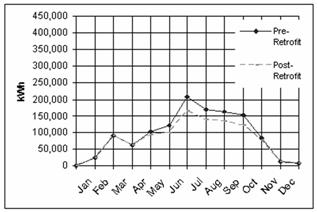
Figure 7: Expected Pre and Post-Retrofit usage for chilled water system retrofit.
Suppose an energy manager replaced the existing chilled water system in a building with a more efficient system. He likely would expect to see energy and cost savings from this retrofit. Figure 7 presents results the energy manager might expect.
But what if, instead, the bills presented the disaster shown in Figure 8?
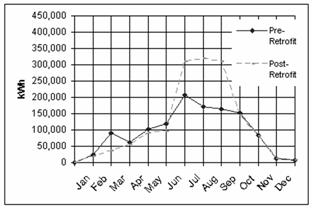
Figure 8: A disaster of a project? Comparison of Pre-Retrofit and Post-Retrofit data
A quarter-million dollar retrofit is difficult to justify with results like this. And yet, the energy manager knows that everything in the retrofit went as planned. What caused these results?
Clearly the energy manager cannot present these results without some reason or justification. Management may simply look at the figures and, since figures don’t lie, conclude they have hired the wrong energy manager!
There are many reasons the retrofit may not have delivered the expected savings. One possibility is that the project is delivering savings, but the summer after the retrofit was much hotter than the summer before the retrofit. Hotter summers translate into higher air conditioning loads, which typically result in higher utility bills.
Hotter Summer -> Higher Air Conditioning Load -> Higher Summer Utility Bills
In other words, the new equipment really did save energy, because it was working more efficiently than the old equipment. The figures don’t show this because this summer was so much hotter than last summer.
If the weather really was the cause of the higher usage, then how could you ever use utility bills to measure savings from energy efficiency projects (especially when you can make excuses for poor performance, like we just did)? Your savings numbers would be at the mercy of the weather. Savings numbers would be of no value at all (unless the weather was the same year after year).
Our example may appear a bit exaggerated, but it begs the question: Could weather really have such an impact on savings numbers?
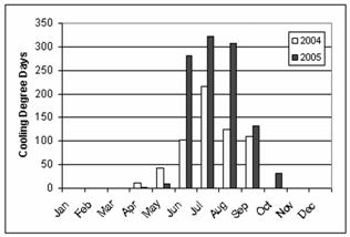
Figure 9: Cooling Degree Days in Detroit, Michigan for 2004 and 2005
It can, but usually not to this extreme. The summer of 2005 was the hottest summer in a century of record-keeping in Detroit, Michigan. There were 18 days at 90°F or above compared to the usual 12 days. In addition, the average temperature in Detroit was 74.8°F compared to the normal 71.4 °F. At first thought, 3 degrees doesn’t seem like all that much; however, if you convert the temperatures to cooling degree days[4], as shown in Figure 9, the results look dramatic. Just comparing the June through August period, there were 909 cooling degree days in 2005 as compared to 442 cooling degree days in 2004. That is more than double! Cooling degree days are roughly proportional to relative building cooling requirements. For Detroit then, one can infer that an average building required (and possibly consumed) more than twice the amount of energy for cooling in the summer of 2005 than the summer of 2004. It is likely that in the Upper Midwestern United States there were several energy managers who faced exactly this problem!
How is an energy manager going to show savings from a chilled water system retrofit under these circumstances? A simple comparison of utility bills will not work, as the expected savings will get buried beneath the increased cooling load. The solution would be to apply the same weather data to the pre- and post-retrofit bills, and then there would be no penalty for extreme weather. This is exactly what weather normalization does. To show savings from a retrofit (or other energy management practice), and to avoid our disastrous example, an energy manager should normalize the utility bills for weather so that changes in weather conditions will not compromise the savings numbers.
More and more energy managers are now normalizing their utility bills for weather because they want to be able to prove that they are actually saving energy from their energy management efforts.
In many software packages, you can establish the relationship between weather and usage in just one click. Because the one-click “tunings” that the software gives you are not always acceptable, it does help to understand the underlying theory and methodology so that you can identify the problem tunings and make the necessary adjustments. The more you know about the topic the better. The section that follows explains in a little more detail the basic elements of weather normalization.
How Weather Normalization Works
Rather than compare last year’s usage to this year’s usage, when we use weather normalization, we compare how much energy we would have used this year to how much energy we did use this year. Many in our industry do not call the result of this comparison, “Savings”, but rather “Usage Avoidance” or “Cost Avoidance” (if comparing costs). Since we are trying to keep this treatment at an introductory level, we will simply use the word Savings.
When we tried to compare last year’s usage to this year’s usage, we saw the disastrous project in Figure 8. We used the equation:
Savings = Last year’s usage – This year’s usage
When we normalize for weather, the same data results in Figure 10 and uses the equation:
Savings = How much energy we would have used this year – This year’s usage
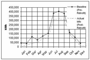
Figure 10: Comparison of Baseline and Actual (Post-Retrofit) data with Weather Correction
The next question is how to figure out how much energy we would have used this year? This is where weather normalization comes in.
First, we select a year of utility bills[5] to which we want to compare future usage. This would typically be the year before you started your energy efficiency program, the year before you installed a retrofit, or some year in the past that you want to compare current usage to. In this example, we would select the year of utility data before the installation of the chilled water system. We will call this year the Base Year[6].
Next, we calculate degree days for the Base Year billing periods. Because this example is only concerned with cooling, we need only gather Cooling Degree Days.
Base Year bills and Cooling Degree Days are then normalized by number of days, as shown in Figure 11. Normalizing by number of days (in this case, merely, dividing by number of days) removes any noise associated with different bill period lengths. This is done automatically by canned software and would need to be performed by hand if other means were employed.
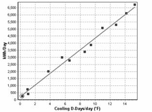
Figure 11: Comparison of Baseline and Actual (Post-Retrofit) data with Weather Correction
To establish the relationship between usage and weather, we find the line that comes closest to all the bills. This line, the Best Fit Line, is found using statistical regression techniques available in canned utility bill tracking software and in spreadsheets.
The next step is to ensure that the Best Fit Line is good enough to use. The quality of the best fit line is represented by statistical indicators, the most common of which, is the R2 value. The R2 value represents the goodness of fit, and in energy engineering circles, an R2 > 0.75 is considered an acceptable fit. Some meters have little or no sensitivity to weather or may have other unknown variables that have a greater influence on usage than weather. These meters may have a low R2 value. You can generate R2 values for the fit line in Excel or other canned utility bill tracking software.
This Best Fit Line has an equation, which we call the Fit Line Equation, or in this case the Baseline Equation. The Fit Line Equation from Figure 11 might be:
Baseline kWh = (5 kWh/Day * #Days ) + ( 417 kWh/CDD * #CDD )[7]
Once we have this equation, we are done with the regression process.
Base Year bills ≈ Best Fit Line = Fit Line Equation
The Fit Line Equation represents how your facility used energy during the Base Year, and would continue to use energy in the future (in response to changing weather conditions) assuming no significant changes occurred in building consumption patterns.
Once you have the Baseline Equation, you can determine if you saved any energy. How? You take a bill from some billing period after the Base Year. You then plug in the number of days from your bill and the number of Cooling Degree Days from the billing period into your Baseline Equation.
Suppose for a current month’s bill, there were 30 days and 100 CDD associated with the billing period.
Baseline kWh = ( 5 kWh/Day * #Days ) + ( 417 kWh/CDD * #CDD )
Baseline kWh = ( 5 kWh/Day * 30 ) + ( 417 kWh/CDD * 100 )
Baseline kWh = 41,850 kWh
Remember, the Baseline Equation represents how your building used energy in the Base Year. So, with the new inputs of number of days and number of degree days, the Baseline Equation will tell you how much energy the building would have used this year based upon Base Year usage patterns and this year’s conditions (weather and number of days). We call this usage that is determined by the Baseline Equation, Baseline Usage.
Now, to get a fair estimate of energy savings, we compare:
Savings = How much energy we would have used this year – How much energy we did use this year
Or if we change the terminology a bit:
Savings = Baseline Energy Usage – Actual Energy Usage
Where Baseline Energy Usage is calculated by the Baseline Equation, using current month’s weather and number of days, and Actual Energy Usage is the current month’s bill.
So, using our example, suppose this month’s bill was for 30,000 kWh:
Savings = Baseline Energy Usage – Actual Energy Usage
Savings = 41,850 kWh – 30,000 kWh
Savings = 11,850 kWh
Summary
Utility Bill Tracking is at the center of a successful energy management system, but the bills must be used for sound analysis for any meaningful reduction in energy usage. By applying three analysis methods presented here (Benchmarking, Load Factor Analysis, and Weather Normalization), the energy manager can develop insight which should lead to sound energy management decisions.
About The Author
John Avina, Director of Abraxas Energy Consulting, has worked in energy analysis and utility bill tracking for over a decade. During his tenure at Thermal Energy Applications Research Center, Johnson Controls, SRC Systems, Silicon Energy and Abraxas Energy Consulting, Mr. Avina has managed the M&V for a large performance contractor, managed software development for energy analysis applications, created energy analysis software that is commercially for sale, taught over 200 energy management classes, created hundreds of building models and utility bill tracking databases, modeled hundreds of utility rates, and set up and maintained M&V projects for a handful of 500 to 1000 unit big box store chains. Mr. Avina has a MS in Mechanical Engineering from the University of Wisconsin-Madison. He is a member of the American Society of Heating, Refrigerating and Air-Conditioning Engineers (ASHRAE), the Association of Energy Engineers (AEE) and a Certified Energy Manager (CEM).
Abraxas Energy Consulting provides utility bill tracking and energy management services for its clients world-wide. In addition to providing the right utility bill tracking software packages for its clients, Abraxas Energy Consulting creates, maintains and analyzes utility bill tracking databases, trains its customers in energy analysis and software, and performs energy audits, LEED studies, and M&V for ESCOs and facility managers.
[1] HDD = Heating Degree Days, CDD = Cooling Degree Days
[2] Load Factors are an excellent tool identifying metering or billing errors. Load Factors greater than 1 are more common than you would think, and are the result of metering or billing problems.
[3] Weather Normalization is more complex than the other methods presented here, and requires more understanding than what is presented here. This paper intends only to present the case for weather normalization.
[4] Cooling Degree Days are a rough measure of how much a period’s weather should result in a building’s cooling requirements. A hotter day will result in more Cooling Degree Days; whereas a colder day may have no Cooling Degree Days. Doubling the amount of cooling degrees should result in roughly double the cooling requirements for a building. Cooling Degree Days over a month or billing period are merely a summation of the Cooling Degree Days calculated for the individual days. Heating Degree Days are like Cooling Degree Days except they relate to heating and not cooling.
[5] Some energy professionals select 2 years of bills rather than one. Good reasons can be argued for either case. Do not choose periods of time that are not in intervals of 12 months (for example, 15 months or 8 months could lead to inaccuracy).
[6] Please do not confuse Base Year with Baseline. Base Year is a time period, from which bills were used to determine the building’s energy usage patterns with respect to weather data, whereas Baseline, as will be described later, represents how much energy we would have used this month, based upon Base Year energy usage patterns and current month conditions (i.e. weather and number of days in the bill).
[7] The generic form of the equation is:
Baseline kWh = (constant * #Days) + (coefficient * #CDD)
where the constant and coefficient (in our example) are 5 and 417.