
August 5, 2009
Abstract
Utility bill tracking is at the heart of an effective energy management program. Merely comparing utility bills can yield inaccurate indications of the amount of savings from energy management programs due to the unaccounted influence of weather or other factors. Correcting utility bills for weather data will give more accurate representations of savings that were accrued. This paper presents the how and why of weather correction for those who want to become more familiar with the concepts and methodology.
What Utility Bill Tracking Can Do For You
Jim Faes from Jefferson County School District wrote:
“Energy accounting is the backbone of our school district’s energy management program.”
Why would he write that? An energy accounting system is much like an airplane’s control panel. In order to correctly navigate your airplane, you need to understand where it is, where it was and where it is going. If you fly the plane without the control panel, you have a good chance of crashing the plane. It is the same with energy management. You need to know where you are, where you were, where you are going, and how where you are now fits with expectations of your progress.
What Utility Bill Tracking Systems Can Do
With utility bill tracking systems, Energy managers can:
- Enter target usage and costs and track their actual performance against their targets
- Discover large increases in energy usage and take corrective actions
- Identify the buildings that are using more $/SQFT than the others, and concentrate energy management activities on those buildings.
- Determine whether your meters are on the best rates
- Check to see if you are being billed correctly by the utility
- Create bills for your tenants (if you have any)
- Determine whether you have saved any energy from your energy conservation measures
- Aggregate your usage and costs and pass this aggregated data to potential energy suppliers
- Create utility budgets
More generally, if you keep aware of the state of your utility accounting, you will know where your facility is and how it is faring towards your goals.
Utility Bill Tracking: The Report Card for Facilities and Facility Managers
Energy Managers and some Facility Managers all to often have to justify their existence to management. How much did we save last year? Is that more than what we pay our energy manager? Did your recommendations give reasonable paybacks? Why do we even have an energy manager?
There are several methods to determine whether you have saved energy from your energy conservation efforts, as described in the literature. You can wave your hands in the air, and decide upon a number; calculate your savings based upon data logger and control points; compare utility bills to determine savings; and finally, employ a building model. (These are referred to as Option A, B, C and D in the IPMVP, FEMP Guidelines and other literature. )
Most likely, the simplest and most palatable method for the facility manager to determine whether you are saving energy is Option C, comparing utility bills. Why? Well, although some utility managers do present calculations given to them by the friendly sales rep, this method is hardly reliable, as they may produce inflated numbers. Placing dataloggers and using existing control points seems easy enough, but converting these inputs into savings numbers can sometimes prove to be outside of the scope of the facility manager’s skillset. Building modeling, while it can be useful, requires hours of time to construct the model, and may represent how much the building should be using, and may not really represent what the building truly is using. If those objections hold, that leaves utility bills as the last remaining method to quantify your performance as an energy manager. Plus, in the end, it is all about the utility bills, as the bills reflect how much you are paying.
Since most facility managers are already tracking their utility bills, it is only one additional small step to see whether you have saved any energy and costs from your energy management program. Just compare prior year bills to current year’s bills, and you will see if you have saved. Well, it isn’t that easy. Let’s find out why.
Why Bill Comparison Doesn’t Work, or, Why Use Weather Correction
Suppose you want to see savings from the new efficient chilled water system you installed this January. A simple comparison of prior and post bills should show the savings right? Well, not exactly. Suppose last year had a relatively cool summer, and this summer was devilishly hot. Would you see the savings? Maybe not.
There are a couple of ways we can plot the usage from year to year. Suppose we just looked at the usage vs. time, like most people do.
Figure 1. One Year of Usage vs. Time (for a real hospital mechanical plant electricity meter) separated out into weather sensitive and non-weather sensitive portions.
We have marked two regions in Figure 1. The bottom (darker) region, we call non-weather sensitive usage. This usage can be attributed to computers, lights, constant volume pumps and other loads that are on regardless of what the weather is. For an all year operation, this amount is steady. (In this case, the non-weather sensitive usage is very low, since this meter serves a mechanical plant. Typically, the non-weather sensitive usage would be higher. )
We call the top (lighter) region weather sensitive usage. This is usage directly related to, in this case, air conditioning the facility. Usage in this region could be attributed to chillers, cycling chilled water pumps, cooling towers, condenser water pumps, condenser fans, and possibly fans and pumps that cycle or are on a variable frequency drive.
If last summer was cool, and this summer was hot, then the non-weather sensitive usage would likely not change from year to year, but the weather sensitive usage would change. Figure 2 is the same as Figure 1, except that it presents 2 years of data. Notice how in the second year, the weather sensitive portion is much greater due to the hot summer’s increased cooling load.
Figure 2. Two Years of Usage vs. Time (for a real hospital mechanical plant electricity meter) separated out into weather sensitive and non-weather sensitive portions
Now suppose that the new chilled water system reduced weather sensitive consumption by 20%. With the weather variation shown in Figure 2, an annual comparison of the usage may not show any energy savings at all, as we can see in Figure 3. (In Figure 3, we removed 20% of the weather sensitive usage from 2002 data, which is what we might see with a chilled water system retrofit. )
Figure 3. A disaster of a project? Comparison of Pre-Retrofit (2001) and Post-Retrofit (2002) Data (assuming chilled water system saved 20% of Post-Retrofit weather sensitive usage).
Imagine showing management these results after you invested a half million dollars. It is hard to inspire confidence in management with graphs like Figure 3. So much for utility bill comparison.
To explain these results, you might provide them with a graph of CDDs (as in Figure 4), and then they could see that, the post-retrofit year (2002) was indeed much hotter, and required more cooling and therefore led to increased usage. This might let you off the hook, but you still need to quantify how much you saved, don’t you? Management will only accept arm waving for so long.
Figure 4. Comparison of Pre-Retrofit and Post-Retrofit CDDs
You can quantify your savings by correcting your utility bill savings equation for weather. Had you done so you could have presented Figure 5, rather than Figure 3.
Figure 5. Same Project, not a disaster after all. Comparison of Baseline and Actual (2002) Data (assuming chilled water system saved 20% of Post-Retrofit weather sensitive usage).
How Weather Correction Works
Rather than compare last year’s usage to this year’s usage, when we use weather correction, we compare how much energy we would have used this year to how much energy we did use this year. Many in our industry do not call the result of this comparison, Savings, but rather Usage Avoidance or Cost Avoidance. But, since we are trying to keep this paper at an introductory level, we will use the word Savings.
When we tried to compare last year’s usage to this year’s usage, we saw Figure 3, and a disastrous project. We used the equation:
Savings = (last year’s usage) – (this year’s usage)
When we use weather correction, we end up with Figure 5, and use the equation:
Savings = (How much energy we would have used this year) – (how much energy we did use this year**)
**where this year’s usage from the 1st equation is the same as how much energy we did use this year from the 2nd equation
The next question is, how do we figure out how much energy we would have used this year. This is done using weather correction as shown below.
First, we select a year of utility bills we want to compare future usage to. This would typically be the year before you started your energy efficiency program, or the year before you, the new facility manager, were hired, or some chosen year. In this example, we would select the year of utility data before the installation of the chilled water system. We will call this year the Base Year.
As shown in Figure 6, we graph Base Year usage versus weather (in the form of Cooling Degree Days or Heating Degree Days). The blue dots represent the utility bills. [1]
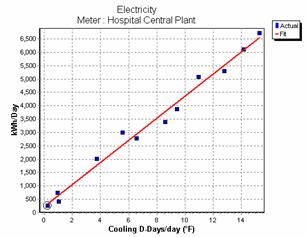
Figure 6. Finding the relationship between usage and weather data.
Then we find the Best Fit Line between usage and weather. The Best Fit Line is the line that comes closest to all the utility bills as shown in Figure 6. We can tell it is the Best Fit Line by looking at some statistical indicators (such as R2 value, Net Mean Bias Error and CVRMSE, which are not covered in this introductory paper). [2]
This Best Fit Line has an equation, which we call the Fit Line Equation, or in this case the Baseline Equation. [3] Once we have this equation, we are done with this regression process. [4]
Review
Let’s recap what we have done thus far:
- We graphed a Base Year of utility data versus weather data
- We found a Best Fit Line through the data. The Best Fit Line then represents the utility bills.
- The Best Fit Line Equation, which represents the Best Fit Line, which in turn represents the Base Year of utility data. The Fit Line Equation represents how your facility used energy during the Base Year, and would continue to use energy in the future (varying with changing weather conditions) assuming there were no significant changes occurred in building consumption patterns, such as new equipment, area or operating hours.
Base Year Bills ┰ˆ Best Fit Line = Fit Line Equation
In our example:
Baseline Equation = Fit Line Equation
Determining If You Saved Energy
Once you have the Baseline Equation, you can determine if you saved any energy. How? You take a bill from some billing period after the Base Year. You (or your software) plug in the number of days and the number of degree days from the bill into your Baseline Equation. Remember, the Baseline Equation represents how your building used to use energy in the Base Year. So, with the new inputs of number of days and number of degree days, the Baseline Equation will tell you how much energy the building would have used this year based upon Base Year usage patterns and this years conditions (weather and number of days). We call this usage that is determined by the Baseline Equation, Baseline Usage.
Now, to get a fair comparison of this year versus last year, we compare:
Savings = (How much energy we would have used this year) – (How much energy we did use this year)
or if we change the terminology a bit:
Savings = (Baseline Energy Usage) – (Actual Energy Usage)
where Baseline Energy Usage is calculated using the Baseline Equation and current month’s weather and number of days, and Actual Energy Usage is the current month’s bill. Both equations are one and the same, Baseline = How much energy we would have used this year, and Actual represents how much energy we did use this year.
Correcting For Other Variables
Facility Managers in the industrial sector may want to correct for production rather than (or in addition to) weather data. This works if you have a simple variable that quantifies your production. For example, an automobile manufacturing plant can track number of automobiles produced. If your factory makes several different things, for example, disk drives, desktop computers, printers and main frame computers, it is difficult to come up with a single variable that could be used to represent production for the entire plant. However, if your printer manufacturing unit was served by a different meter or submeter than the other units, then you could use the number of printers produced as a variable for the meter (or submeter) that serves the printing unit.
Weather Correction In Excel vs. Canned Software
Weather correction can be done in Excel, however it can be laborious, and oftentimes may not be as rigorous as when done using specialized software. Excel will give regressions, fit line equations, and statistical indicators which show how well your usage is represented by the fit line. However, it is difficult to find the best balance point in Excel, as you can in specialized software. Excel may force you have to choose just one balance point, and possibly then you would iterate with different balance points, whereas canned software will allow you to easily find the best fit line using different balance points. In addition, if you enter your weather data in high low temperatures or average temperatures, it can be difficult to apply the correct weather data to the correct billing periods. Try it, and you will see.
Available Weather Correction Desktop Software
All of the major desktop utility bill tracking software packages will now correct for weather data. Nearly all of them will correct for your own variables as well. The major desktop programs are EnergyCAP®, Metrix┞¢, Stark Essentials┞¢. You can find information on all of them online.
Conclusion
Weather changes from year to year. If wish to use utility bills to show energy savings from energy management programs with any degree of accuracy, it is important to correct your utility bills for fluctuations in weather.
About The Author
John Avina, Director of Abraxas Energy Consulting, has worked in energy analysis and utility bill tracking for over a decade. Mr. Avina performed M&V for Performance Contracting at Johnson Controls. Then as Manager of Technical Services at SRC Systems, he taught well over 100 software classes, handled technical support, assisted with product development, and wrote manuals for Metrix Utility Accounting System┞¢. When SRC Systems merged with Silicon Energy Inc. , Mr. Avina managed the development of new analytical software that employed the weather regression algorithms found in Metrix┞¢. In October 2001, Mr. Avina, and others from the defunct SRC Systems, founded Abraxas Energy Consulting. Mr. Avina has a MS in Mechanical Engineering from the University of Wisconsin-Madison, where he was a research assistant at the Solar Energy Lab. He is a Member of the American Society of Heating Refrigeration and Air-Conditioning Engineers (ASHRAE), the Association of Energy Engineers (AEE), and a Certified Energy Manager (CEM).
Abraxas Energy Consulting (www.abraxasenergy.com) sells all of the major utility bill tracking software programs, including EnergyCAP® Enterprise, Metrix┞¢, Stark Essentials┞¢. Abraxas Energy Consulting specializes in finding the right utility bill tracking program for their clients. The company also provides engineering services such as bill tracking, creation of bill tracking databases, energy audits and related customized software applications.
[1] Cooling Degree Days are a simplified measure of how much cooling would likely be needed by a building for a period of time, such as a billing period. If you were calculating Cooling Degree Days for a billing period, then you would calculate Cooling Degree Days for each day and sum them up over the billing period. Cooling Degree Days are calculated for each day using the equation: CDD = [(Thi – Tlo)/2 – TBP ] x 1 Day, where Thi = the daily high temperature, and Tlo is the daily low temperature, and TBP is the building’s balance point temperature. In the past 65oF was considered a balance point acceptable for all buildings, but now engineers recognize that every building is different, and has its own balance point.
[2] The simplest statistical indicator to use is the R2 value, which represents the goodness of fit. In our industry, an R2 value above 0. 75 is considered an acceptable fit. Some meters have little or no sensitivity to weather, and would have a low R2 value. You can generate R2 values for the fit line in Excel or other canned utility bill tracking software.
[3] Baseline Equation = Fit Line Equation +/- Baseline Modifications.
[4] There are several names for this process of finding the best fit line. Other names include “Tuning”, “Performing a Regression”, “Regressing bill data to weather data”